Example of a Simulated Gamma-Poisson Model

Usage

example_hmm_mcmc_gamma_poisson

Format

hmm_mcmc_gamma_poisson object

Examples

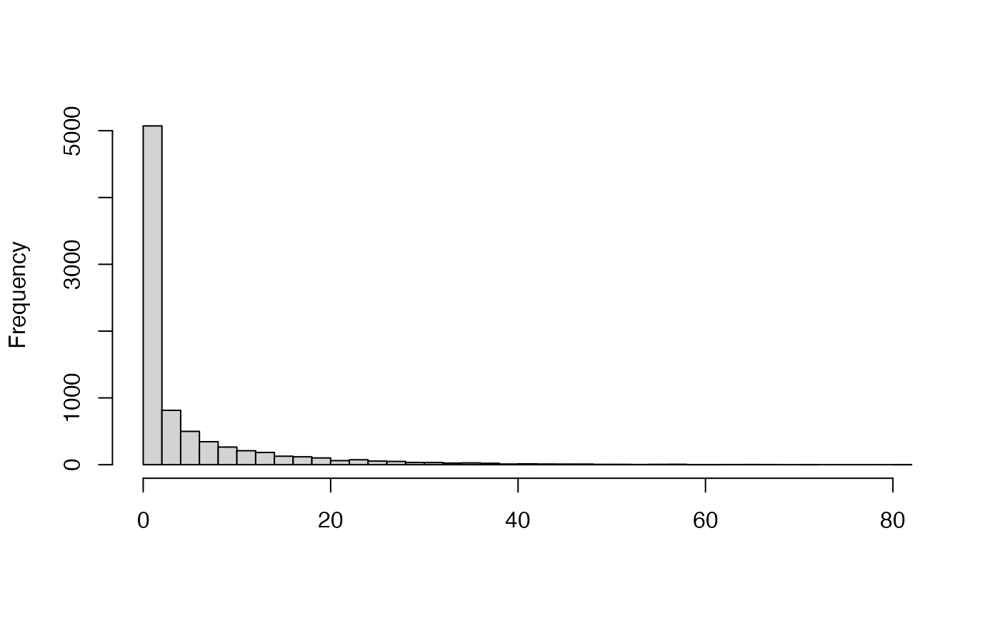
# Data stored in the object
hist(example_hmm_mcmc_gamma_poisson$data, 
     breaks = 50, xlab = "", main = "")


# Priors used in simulation
example_hmm_mcmc_gamma_poisson$priors
#> $prior_betas
#> [1] 5 3 1
#> 
#> $prior_alpha
#> [1] 1.047478
#> 
#> $prior_T
#>           [,1]      [,2]      [,3]
#> [1,] 0.2611659 0.7388341 0.0000000
#> [2,] 0.2607206 0.4662956 0.2729838
#> [3,] 0.0000000 0.2181791 0.7818209
#> 

# Model
example_hmm_mcmc_gamma_poisson
#> Model: HMM Gamma-Poisson 
#> Type: MCMC 
#> Iter: 1500 
#> Warmup: 600 
#> Thin: 1 
#> States: 3 

summary(example_hmm_mcmc_gamma_poisson)
#> Estimated betas:
#>   beta[1]   beta[2]   beta[3] 
#> 5.5567893 0.6803553 0.1114030 
#> 
#> Estimated alpha:
#> 1.302679
#> 
#> Estimated means:
#> 0.234817 1.915574 11.69664
#> 
#> Estimated transition rates:
#>            1          2          3
#> 1 0.98701139 0.01298861 0.00000000
#> 2 0.01237949 0.97545367 0.01216684
#> 3 0.00000000 0.01201136 0.98798864
#> 
#> Number of windows assigned to hidden states:
#>    1    2    3 
#> 2640 2748 2804 
#> 
#> Kullback-Leibler divergence between observed and estimated distributions:
#> 0.03197473
#> 
#> Log Likelihood:
#>          mean            sd        median 
#> -16995.384239      1.407003 -16995.160683 
#> 
#> P-value of poisson test for difference between rates of states (stepwise):
#> 1-2 2-3 
#>   0   0 
#>