MCMC Sampler for the Hidden Markov Model with Normal emission densities

Usage

hmm_mcmc_normal(
  data,
  prior_T,
  prior_means,
  prior_sd,
  iter = 600,
  warmup = floor(iter/5),
  thin = 1,
  seed = sample.int(.Machine$integer.max, 1),
  init_T = NULL,
  init_means = NULL,
  init_sd = NULL,
  print_params = TRUE,
  verbose = TRUE
)

Arguments

data: (numeric) normal data
prior_T: (matrix) prior transition matrix
prior_means: (numeric) prior means
prior_sd: (numeric) a single prior standard deviation
iter: (integer) number of MCMC iterations
warmup: (integer) number of warmup iterations
thin: (integer) thinning parameter. By default, 1
seed: (integer) optional parameter; seed parameter
init_T: (matrix) optional parameter; initial transition matrix
init_means: (numeric) optional parameter; initial means
init_sd: (numeric) optional parameter; initial standard deviation
print_params: (logical) optional parameter; print parameters every iteration. By default, TRUE
verbose: (logical) optional parameter; print additional messages. By default, TRUE

Value

List with following elements:

data: data used for simulation
samples: list with samples
estimates: list with various estimates
idx: indices with iterations after the warmup period
priors: prior parameters
inits: initial parameters
last_iter: list with samples from the last MCMC iteration
info: list with various meta information about the object

Details

Please see supplementary information at doi:10.1186/s12859-024-05751-4 for more details on the algorithm.

For usage recommendations please see https://github.com/LynetteCaitlin/oHMMed/blob/main/UsageRecommendations.pdf.

References

Claus Vogl, Mariia Karapetiants, Burçin Yıldırım, Hrönn Kjartansdóttir, Carolin Kosiol, Juraj Bergman, Michal Majka, Lynette Caitlin Mikula. Inference of genomic landscapes using ordered Hidden Markov Models with emission densities (oHMMed). BMC Bioinformatics 25, 151 (2024). doi:10.1186/s12859-024-05751-4

Examples

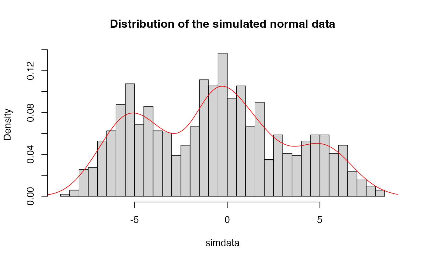
# Simulate normal data
N <- 2^10
true_T <- rbind(c(0.95, 0.05, 0),
                c(0.025, 0.95, 0.025),
                c(0.0, 0.05, 0.95))

true_means <- c(-5, 0, 5)
true_sd <- 1.5

simdata_full <- hmm_simulate_normal_data(L = N, 
                                         mat_T = true_T, 
                                         means = true_means,
                                         sigma = true_sd)
simdata <- simdata_full$data
hist(simdata, 
     breaks = 40, 
     probability = TRUE,  
     main = "Distribution of the simulated normal data")
lines(density(simdata), col = "red")


# Set numbers of states to be inferred
n_states_inferred <- 3

# Set priors
prior_T <- generate_random_T(n_states_inferred)
prior_means <- c(-18, -1, 12)
prior_sd <- 3

# Simmulation settings
iter <- 50
warmup <- floor(iter / 5) # 20 percent
thin <- 1
seed <- sample.int(10000, 1)
print_params <- FALSE # if TRUE then parameters are printed in each iteration
verbose <- FALSE # if TRUE then the state of the simulation is printed

# Run MCMC sampler
res <- hmm_mcmc_normal(data = simdata,
                       prior_T = prior_T,
                       prior_means = prior_means,
                       prior_sd = prior_sd,
                       iter = iter,
                       warmup = warmup,
                       seed = seed,
                       print_params = print_params,
                       verbose = verbose)
res
#> Model: HMM Normal 
#> Type: MCMC 
#> Iter: 50 
#> Warmup: 10 
#> Thin: 1 
#> States: 3 

summary(res) # summary output can be also assigned to a variable
#> Estimated means:
#>   mean[1]   mean[2]   mean[3] 
#> -4.984660  1.457898  1.727691 
#> 
#> Estimated standard deviation:
#> 2.464708
#> 
#> Estimated transition rates:
#>            1          2         3
#> 1 0.95361104 0.04638896 0.0000000
#> 2 0.05236891 0.03687321 0.9107579
#> 3 0.00000000 0.82080504 0.1791950
#> 
#> Number of windows assigned to hidden states:
#>   1   2   3 
#> 357 276 391 
#> 
#> Approximate Kullback-Leibler divergence between observed and estimated distributions:
#> 0.0155315
#> 
#> Log Likelihood:
#>        mean          sd      median 
#> -2470.73655     1.76743 -2470.62543 
#> 
#> P-value of t-test for difference between means of states (stepwise):
#>           1-2           2-3 
#> 2.734115e-155  8.292237e-10 
#> 

coef(res) # extract model estimates
#> $means
#>   mean[1]   mean[2]   mean[3] 
#> -4.984660  1.457898  1.727691 
#> 
#> $sd
#> [1] 2.464708
#> 
#> $mat_T
#>            [,1]       [,2]      [,3]
#> [1,] 0.95361104 0.04638896 0.0000000
#> [2,] 0.05236891 0.03687321 0.9107579
#> [3,] 0.00000000 0.82080504 0.1791950
#> 

# plot(res) # MCMC diagnostics