Simulate data distributed according to oHMMed with gamma-poisson emission densities

Usage

hmm_simulate_gamma_poisson_data(L, mat_T, betas, alpha)

Arguments

L: (integer) number of simulations
mat_T: (matrix) a square matrix with the initial state
betas: (numeric) rate parameter in rgamma for emission probabilities
alpha: (numeric) shape parameter in rgamma for emission probabilities

Value

Returns a list with the following elements:

data: numeric vector with data
states: an integer vector with "true" hidden states used to generate the data vector
pi: numeric vector with prior probability of states

Examples

mat_T <- rbind(c(1-0.01, 0.01, 0),
               c(0.01, 1-0.02, 0.01),
               c(0, 0.01, 1-0.01))
L <- 2^7
betas <- c(0.1, 0.3, 0.5)
alpha <- 1

sim_data <- hmm_simulate_gamma_poisson_data(L = L,
                                            mat_T = mat_T,
                                            betas = betas,
                                            alpha = alpha)
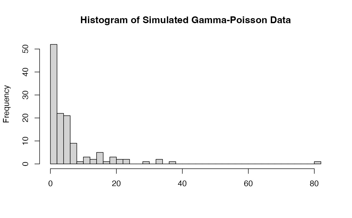
hist(sim_data$data, 
     breaks = 40,
     main = "Histogram of Simulated Gamma-Poisson Data", 
     xlab = "")

sim_data
#> $data
#>   [1]  5  9  2  1  1  4  3  0  1  6  3  8  0 11  3  4  5  5  2  0  8  2  1  6  3
#>  [26]  2  0  0  1  0  3  0  4  3  0  0  3  0  5  5  0  4  7  5  4  3  4  1  0  0
#>  [51]  4  2  0  0  0  1  0  2  1  8  1 10 10  4  1  0  0  8  4  2  1  0  0  0  0
#>  [76]  4  5  0  1  2  0  2  0  1  0  1  2 11  3  4  8  1  1  9  4  3 12  1  1  1
#> [101]  0  1  4  0  1 20  1  9 19  9 11 11  7  4 32 14  2  9  8  8 10 13  1  1 22
#> [126] 32  5  2
#> 
#> $states
#>   [1] 3 3 3 3 3 3 3 3 3 3 3 3 3 2 2 2 2 2 2 2 2 2 2 2 2 2 2 2 2 2 2 2 2 2 2 2 2
#>  [38] 2 2 2 2 2 2 2 2 2 2 2 2 2 2 2 2 2 2 2 2 2 2 2 2 2 2 2 2 2 2 2 2 2 2 2 2 2
#>  [75] 2 2 2 2 2 2 2 2 2 2 2 2 2 2 2 2 2 2 2 2 2 2 2 2 2 2 2 2 2 2 1 1 1 1 1 1 1
#> [112] 1 1 1 1 1 1 1 1 1 1 1 1 1 1 1 1 1
#> Levels: 1 2 3
#> 
#> $pi
#> [1] 0.3333333 0.3333333 0.3333333
#>