Forward-Backward Algorithm to Calculate the Posterior Probabilities of Hidden States in Poisson-Gamma Model

Usage

posterior_prob_gamma_poisson(data, pi, mat_T, betas, alpha)

Arguments

data: (numeric) Poisson data
pi: (numeric) prior probability of states
mat_T: (matrix) transition probability matrix
betas: (numeric) vector with prior rates
alpha: (numeric) prior scale

Value

List with the following elements:

F: auxiliary forward variables
B: auxiliary backward variables
s: weights

Details

Please see supplementary information at doi:10.1186/s12859-024-05751-4 for more details on the algorithm.

Examples

mat_T <- rbind(c(1-0.01,0.01,0),
               c(0.01,1-0.02,0.01),
               c(0,0.01,1-0.01))
L <- 2^10
betas <- c(0.1, 0.3, 0.5)
alpha <- 1

sim_data <- hmm_simulate_gamma_poisson_data(L = L,
                                            mat_T = mat_T,
                                            betas = betas,
                                            alpha = alpha)
pi <- sim_data$pi
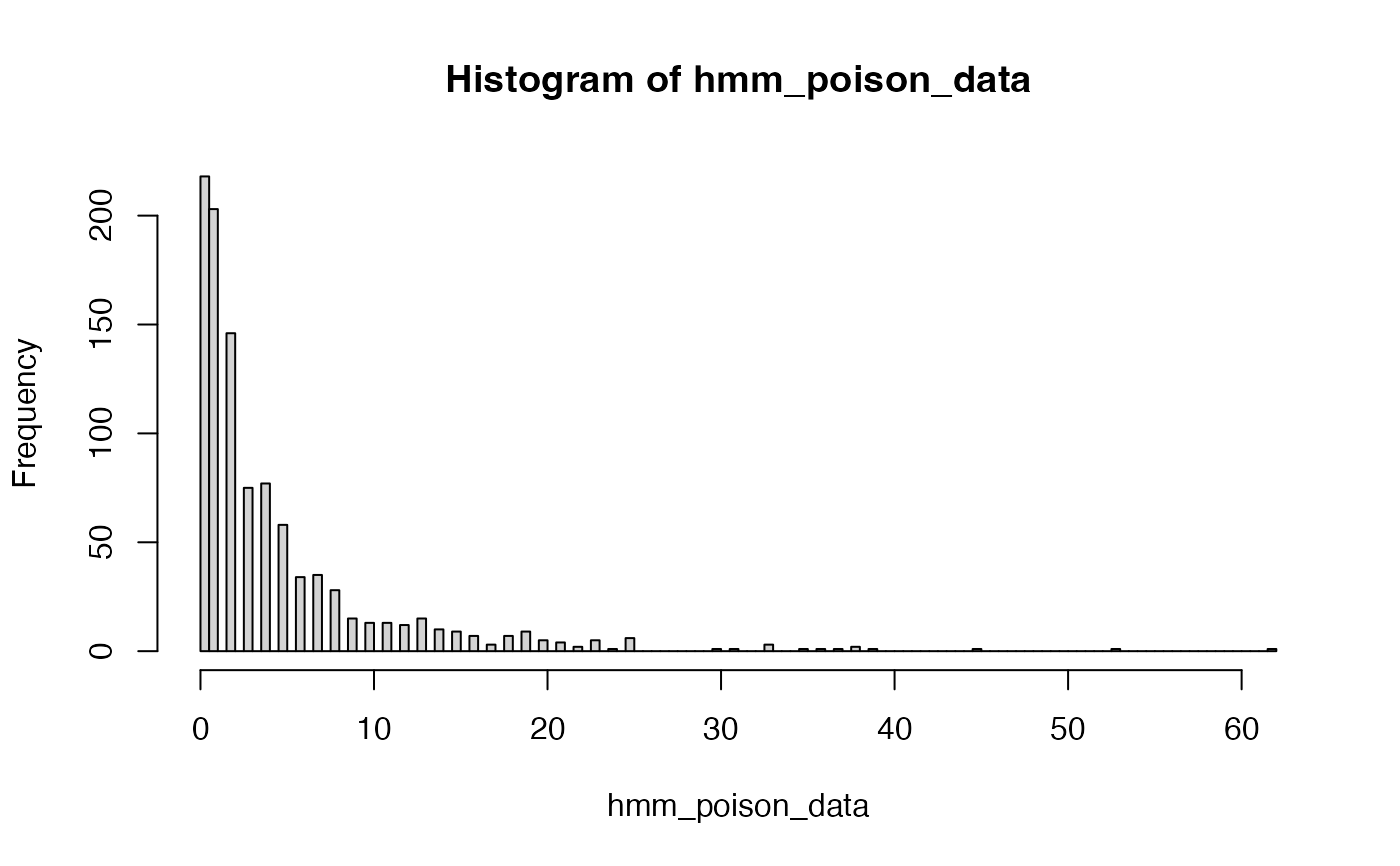
hmm_poison_data <- sim_data$data
hist(hmm_poison_data, breaks = 100)


# Calculate posterior probabilities of hidden states
post_prob <- posterior_prob_gamma_poisson(data = hmm_poison_data,
                                          pi = pi,
                                          mat_T = mat_T,
                                          betas = betas,
                                          alpha = alpha)
str(post_prob)
#> List of 3
#>  $ F: num [1:1024, 1:3] 0.738 0.686 0.441 0.434 0.219 ...
#>  $ B: num [1:1024, 1:3] 4.8379 0.5516 0.1976 0.2955 0.0762 ...
#>  $ s: num [1:1024] 0.0119 0.0663 0.1407 0.0574 0.1803 ...